Most studied worm neuronal genes

worm
R
Author

Alexis Weinreb

Published

November 5, 2023

What genes are the most studied in worms? Wormbase’s comprehensive curation can help us answer that.

Data download

We want to find how many publications are associated with each gene. Wormbase offers us several tools to that effect, we will use SimpleMine which is the easiest here. Other possibilities include WormMine or the REST API.

In a browser, we open SimpleMine. For “Step 1”, we can simply select Caenorhabditis elegans, in “Step 2” we will “download results as a tab-delimited file”, in Step 3 we select “Wormbase Gene ID”, “Public Name”, “Expr_pattern Tissue” and “Reference”. And in Step 4 we download “all genes for this species”.

We can then download the data. We need a tool to process it, here, I will use R.

Data loading

The first step is to read the data into R, we also rename the columns for names that are easier to work with. And if you look through the data, you may notice a number of genes do not have references associated (marked as “N.A.”), we need to ensure this is registered correctly.

suppressPackageStartupMessages(library(tidyverse))

simplemine_results <- read_tsv("data/simplemine_results.txt",
                               col_types = "ccccc",
                               na = "N.A.") |>
  select(gene_id = `WormBase Gene ID`,
         gene_name = `Public Name`,
         expr_pattern = `Expr_pattern Tissue`,
         references = Reference)

simplemine_results
# A tibble: 49,541 × 4
   gene_id        gene_name expr_pattern                              references
   <chr>          <chr>     <chr>                                     <chr>     
 1 WBGene00000001 aap-1     body wall musculature, hypodermis, intes… WBPaper00…
 2 WBGene00000002 aat-1     excretory cell, excretory gland cell, go… WBPaper00…
 3 WBGene00000003 aat-2     <NA>                                      WBPaper00…
 4 WBGene00000004 aat-3     <NA>                                      WBPaper00…
 5 WBGene00000005 aat-4     <NA>                                      WBPaper00…
 6 WBGene00000006 aat-5     <NA>                                      WBPaper00…
 7 WBGene00000007 aat-6     intestine                                 WBPaper00…
 8 WBGene00000008 aat-7     <NA>                                      WBPaper00…
 9 WBGene00000009 aat-8     <NA>                                      WBPaper00…
10 WBGene00000010 aat-9     body wall musculature, neuron             WBPaper00…
# ℹ 49,531 more rows

In this format, the references are all packed in a single long string. We can count how many there are by relying on the consistent format. We just need to handle the case of references being “NA”. R would interpret it as “some unknown number of references”, but we know this actually means “no reference”.

papers_per_gene <- simplemine_results |>
  mutate(nb_papers = str_count(references, "WBPaper\\d{8}"),
         nb_papers = if_else(is.na(references), 0, nb_papers)) |>
  arrange(desc(nb_papers))

papers_per_gene
# A tibble: 49,541 × 5
   gene_id        gene_name expr_pattern                    references nb_papers
   <chr>          <chr>     <chr>                           <chr>          <dbl>
 1 WBGene00000912 daf-16    AIYL, AIYR, anterior distal ti… WBPaper00…      1675
 2 WBGene00000898 daf-2     ADFL, ADFR, amphid neuron, ASH… WBPaper00…      1543
 3 WBGene00001609 glp-1     AB, AB lineage cell, ABa, ABal… WBPaper00…       838
 4 WBGene00000417 ced-3     ABaraapapaa, ABaraapapaad, ABa… WBPaper00…       724
 5 WBGene00004804 skn-1     AB, ABa, ABp, AIYL, AIYR, ante… WBPaper00…       695
 6 WBGene00003001 lin-12    ABplaaa, ABplpapp, ccDL, ccDR,… WBPaper00…       685
 7 WBGene00000090 age-1     accessory cell, amphid neuron,… WBPaper00…       595
 8 WBGene00002335 let-60    AIMR, AIYR, anchor cell, anter… WBPaper00…       566
 9 WBGene00006789 unc-54    anal depressor muscle, anal sp… WBPaper00…       562
10 WBGene00000418 ced-4     anal sphincter muscle, apoptot… WBPaper00…       502
# ℹ 49,531 more rows

Alternatively, an approach that is less efficient here, but maybe more general, is to make it one row per reference and count the number of rows for a given gene.

papers_per_gene2 <- simplemine_results |>
  separate_rows(references, sep = ",") |>
  filter(!is.na(references)) |>
  group_by(gene_id, gene_name) |>
  summarize(nb_papers = n(),
            .groups = "drop") |>
  arrange(desc(nb_papers))

all.equal(papers_per_gene |>
            filter(! is.na(references)) |>
            select(-expr_pattern, -references),
          papers_per_gene2)
[1] TRUE

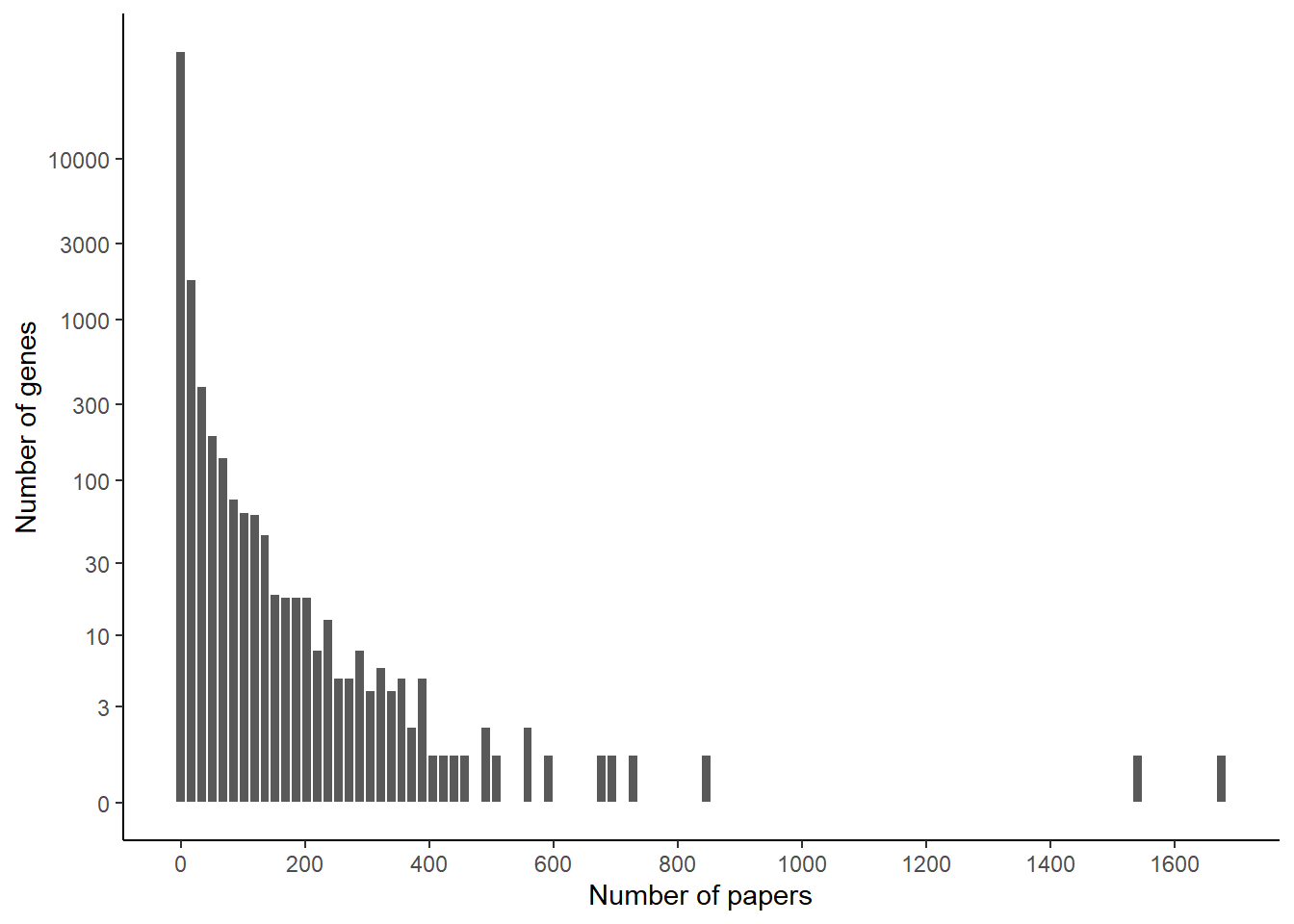
Looking at the top genes, perhaps unsurprisingly, the 2 most studied genes in worms are daf-2 and daf-16. Then we see a lot more genes that also appear widely cited. Let’s look at the distribution to see if we can identify distinct categories.

ggplot(papers_per_gene) +
  geom_histogram(aes(x=nb_papers), bins = 100, color = "white") +
  theme_classic() +
  scale_x_continuous(n.breaks = 10) +
  scale_y_continuous(trans = "log1p", breaks = c(0,3,10,30,100,300,1000,3000,10000)) +
  xlab("Number of papers") + ylab("Number of genes")

So categories we could distinguish are:

  • genes with more than 250 papers, that appeared at the top of the list
  • genes with many papers (let’s take > 20)
  • genes with few or no papers

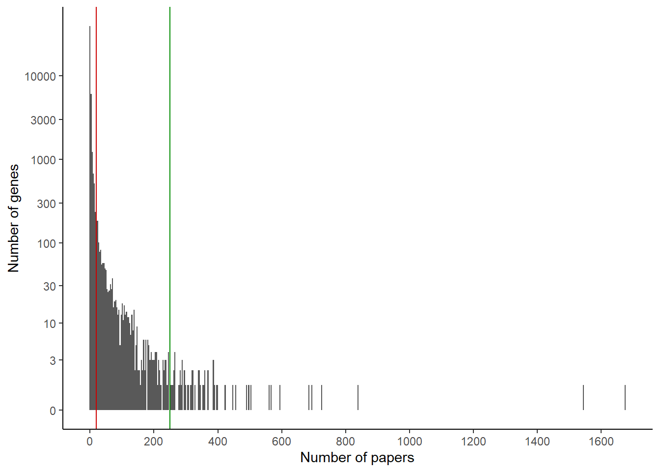
We can visualize these cutoffs on the histogram:

ggplot(papers_per_gene) +
  geom_histogram(aes(x=nb_papers), bins = 500) +
  theme_classic() +
  scale_x_continuous(n.breaks = 10) +
  scale_y_continuous(trans = "log1p", breaks = c(0,3,10,30,100,300,1000,3000,10000)) +
  xlab("Number of papers") + ylab("Number of genes") +
  geom_vline(aes(xintercept = 20), color = "red3") +
  geom_vline(aes(xintercept = 250), color = "green4")

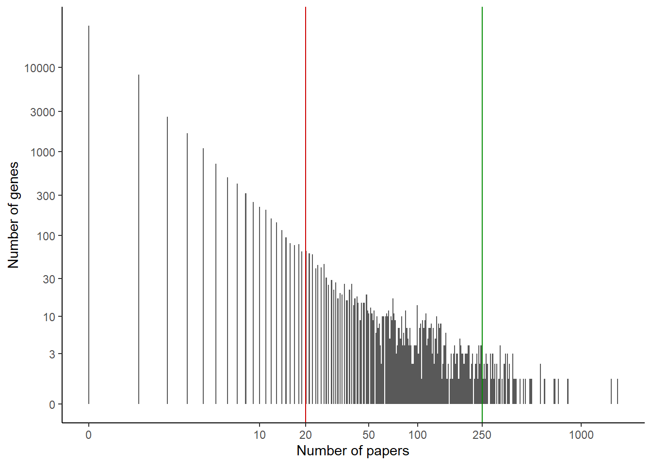
It might help to visualize the x axis on a log scale:

ggplot(papers_per_gene) +
  geom_histogram(aes(x=nb_papers), bins = 500) +
  theme_classic() +
  scale_x_continuous(trans = "log1p", breaks = c(0, 10, 20, 50, 100, 250, 1000)) +
  scale_y_continuous(trans = "log1p", breaks = c(0,3,10,30,100,300,1000,3000,10000)) +
  xlab("Number of papers") + ylab("Number of genes") +
  geom_vline(aes(xintercept = 20), color = "red3") +
  geom_vline(aes(xintercept = 250), color = "green4")

Looking at this graph, maybe a cutoff of 50 genes would be more appropriate than 20. But from domain knowledge, 50 seems too high a cutoff: would we really call a gene with 25 papers poorly studied?

We can look at the number of genes in each category:

papers_per_gene |>
  mutate(category = cut(nb_papers,
                        breaks = c(-1, 3, 20, 250, Inf),
                        labels = c("unstudied", "lowly","medium","highly"))) |> 
  summarize(nb_genes = n(),
            .by = category)
# A tibble: 4 × 2
  category  nb_genes
  <fct>        <int>
1 highly          59
2 medium        1308
3 lowly         4602
4 unstudied    43572

So, there are 59 highly studied genes, and another 1308 well-studied genes. Let’s take a closer look at these most cited genes.

papers_per_gene |>
  filter(nb_papers >= 250) |>
  pull(gene_name)
 [1] "daf-16"  "daf-2"   "glp-1"   "ced-3"   "skn-1"   "lin-12"  "age-1"  
 [8] "let-60"  "unc-54"  "ced-4"   "daf-12"  "let-23"  "daf-7"   "let-7"  
[15] "mab-5"   "unc-6"   "egl-1"   "tra-1"   "fem-3"   "lin-4"   "ced-9"  
[22] "tra-2"   "unc-13"  "unc-22"  "lin-14"  "gld-1"   "lin-3"   "mec-4"  
[29] "mpk-1"   "sod-3"   "goa-1"   "rol-6"   "unc-5"   "lin-15B" "lin-39" 
[36] "par-3"   "daf-4"   "glr-1"   "pop-1"   "unc-40"  "ced-10"  "lin-15A"
[43] "par-2"   "pie-1"   "fem-1"   "unc-104" "clk-1"   "hsf-1"   "unc-4"  
[50] "ced-1"   "egl-5"   "par-1"   "lin-28"  "myo-3"   "tax-4"   "unc-86" 
[57] "lin-17"  "unc-29"  "her-1"  

By tissue type

Let’s say I’m more interested in neuronal genes that are highly studied. One way to implement such a restriction is to look at which tissue each gene is supposedly expressed in.

simplemine_results |>
  mutate(is_neuronal = str_detect(expr_pattern, "neuron")) |>
  filter(is_neuronal) |>
  separate_rows(references, sep = ",") |>
  filter(!is.na(references)) |>
  group_by(gene_id, gene_name) |>
  summarize(nb_papers = n(),
            .groups = "drop") |>
  arrange(desc(nb_papers)) |>
  filter(nb_papers >= 250) |>
  select(gene_name, nb_papers) |>
  knitr::kable()
gene_name nb_papers
daf-16 1675
daf-2 1543
glp-1 838
skn-1 695
lin-12 685
age-1 595
let-60 566
ced-4 502
daf-12 496
let-23 490
daf-7 455
let-7 447
mab-5 423
unc-6 400
tra-1 390
lin-4 386
unc-13 368
lin-14 358
gld-1 355
mec-4 347
mpk-1 343
goa-1 340
unc-5 328
lin-15B 322
lin-39 321
daf-4 319
glr-1 316
pop-1 308
unc-40 305
unc-104 287
hsf-1 282
unc-4 281
ced-1 280
egl-5 266
par-1 266
lin-28 265
tax-4 263
unc-86 261
lin-17 258
unc-29 256

Limitations

First, we are interested in most studied genes, but we only looked at the most cited genes. For example, unc-54 is highly cited, but that may be largely due to its use in transgenes.

Second, for annotating tissue types, we rely on the curated expression patterns from Wormbase. Another approach is to use the scRNA-Seq data now available to determine expression patterns. For example, I previously used a thresholding approach to identify neuronal genes, this annotation is available in the minipackage wormDatasets.

Finally, if we are interested in genes studied for their role in a given tissue (e.g. neurons), we would need a classification of the papers they’re cited in. Here, we rely on (sometimes imprecise) annotations of tissues where a gene is expressed. For example, daf-16 is expressed in neurons, and has been largely studied in all tissues, so it appears as the top hit; that does not necessarily mean it has been studied in neurons that much.